Operations & Production Planning
What to produce, how much, and when. A seasonal forecast built from history instead of gut feel, feeding the production plan.
The system agrees with the hand-built spreadsheet on every variety it was checked against. It works out what to produce from live sales, stock, and incoming orders. It flags shortages early enough to act on a one-year lead time, and lets the planner test a big sale or a capacity drop before any seed is committed.
Built for Veginova, a seed business with a hard constraint: seed takes about a year to produce. The validation in this piece (that the system reproduces the planner’s own numbers, zero mismatches) is real. Where I quote how many varieties were at risk or how much to produce, those figures are real live-snapshot numbers from the build. The system, and the validation that proves it works, are the real ones.
Pillars this case proves: commercial · close to the decision makers · data depth
Situation: one question runs the whole operation
One question runs the whole operation: how much of each variety must we produce, and when do we have to start? The planner asked it every cycle, and leadership stood behind it, because the answer commits seed to a year in the ground. Behind it sit two inputs: how much will we sell of each variety, and how much do we have or already on the way.
Get it wrong in either direction and it costs real money. Produce too little and you miss a year of sales you can’t recover. Produce too much and you tie up cash in seed you don’t need.
Task: make the planner’s hand calculation current and testable
The requirement was not a dashboard. It was a decision: which varieties will run short, and how much of each must be committed to now.
Three constraints shaped it. The output had to match the planner’s own numbers exactly, or it would not be trusted and would not be used. It had to recompute the moment sales or stock changed, because a plan built on last week’s stock is the problem being solved.
And it had to let the planner test a large order or a capacity drop before committing seed, without that test changing anything stored.
What the data looked like before
Production planning ran on a spreadsheet the planner maintained by hand. It worked, until it didn’t. The moment a sale landed or stock changed, the spreadsheet was out of date, and the production decisions built on it were based on stale numbers. The planner was effectively running the whole production, inventory, and sales triangle in their head, cross-referencing sales, stock, and incoming orders by hand.
The stakes are high because of one brutal fact: seed production takes about a year. If you discover you’re short of a variety, it’s already twelve months too late to make more. You can’t react to a stockout. You have to see it coming.
Action: put the planner’s own calculation into a system that updates itself
I took the logic the planner was running by hand and built it into a live system. For every seed variety, it computes the core question, how much to produce, from what’s actually selling, what’s in stock, and what’s already on the way.
The path from source to screen: sales, stock, and incoming orders load automatically from the source sheets into Postgres with Python. The planning logic runs as one SQL view against a proper data model. Power BI is the display layer on top. Building it this way is what lets the plan update itself and stay accurate as sales and stock change.
Three things made it useful beyond the spreadsheet:
- It stays current. When sales or stock change, the plan updates. No manual rebuild.
- It respects the one-year lead time. It flags which varieties are short, and when production has to start to cover each one in time.
- It tests scenarios. The planner can ask “what if sales come in higher,” “what if production capacity drops,” or “what if we lose stock,” and see which varieties go at risk.
The full technical detail (the SQL engine, the snapshot mechanism, the validation gate, the what-if layer) is in “How it’s built” at the bottom.
Result: zero mismatches against the planner’s sheet, enforced on every build
The real test of a planning system is whether it matches reality. I validated the engine against the planner’s own existing spreadsheet, the numbers built by hand over years of running the business.
It reproduced the planning figures exactly, with zero mismatches. That’s what made it trustworthy: it wasn’t a different answer, it was the planner’s answer, made live and able to update itself. A planner doesn’t adopt a system that argues with them. They adopt one that agrees with the sheet they trust, and then keeps up when the sheet can’t.
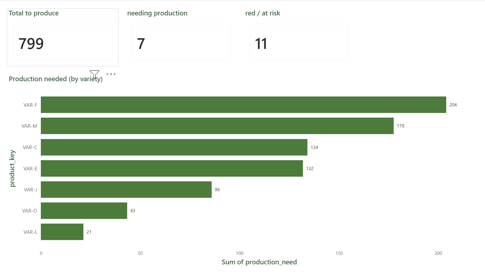 The production plan: total to produce, varieties needing production, and varieties at risk, with the produce quantity per variety. The planner’s red/green sheet, made live and always current. The real Power BI dashboard, shown on illustrative data.
Across the active varieties, the live snapshot showed 500 units to produce, 13 varieties red (below the safety line), and 9 needing production this cycle. Two of those numbers look like they should match but don’t, and the gap is the point: a variety can be red (its ending stock is below the safety line) yet still need zero production, because it has enough to cover its own expected sales. The system shows both, so a warning light is never mistaken for a production order.
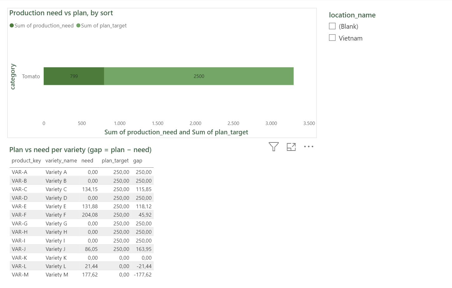 Computed need beside the planner’s own batch target, variety by variety, so the gap between “just enough” and the planner’s lot size is visible, not buried. The real Power BI dashboard, shown on illustrative data.
What changed
- Production decisions from live data, not a stale spreadsheet. The plan shows what’s actually happening, not last month’s snapshot.
- Stockouts visible before they’re unfixable. With a one-year lead time, seeing a shortage early is the entire game. It’s the difference between covering it and missing a year of sales.
- The manual spreadsheet work each planning cycle largely disappears. The system maintains the plan that used to be rebuilt by hand.
- Scenario testing lets the planner pressure-test a decision (a big order, a capacity problem, a stock loss) before committing seed to a year in the ground.
The planner runs production off a system that updates itself and shows what’s at risk before it’s too late to act. They can commit production decisions with confidence, see months ahead which varieties will run short, and test the impact of a big sale or a capacity problem before it happens, instead of finding out a year later.
What it does not do
This is not statistical forecasting. It is a planning system with scenario testing, validated against ground truth. The business runs on named deals, not predictable trends, so the planner’s judgment is the input and the system makes that judgment live, fast and forward-looking. Claiming a forecast the data can’t support would be the weaker move.
Production is never measured. implied_production is inferred from stock movement. When stock rises with no recorded arrival, the system attributes the difference to production. That is an inference, and where it comes out negative the transparency page flags it rather than absorbing it.
Stock history is two observations. Everything drawn between them is interpolation. The line looks like a trend and is not one. It is two audited year-ends with a straight line between them.
The safety buffer is unseeded. safety_floor and safety_months have no per-variety values yet, so the engine currently produces just enough not to go negative rather than a real batch size. Setting them is a growing decision, not a modelling one I can make.
Year two is built and unvalidated. The multi-year view’s first year is checked against the live plan. The recursion beyond it runs, but only one sales year is seeded, so it has never been proven.
Stack and role
Built end-to-end, solo, close to the decision makers. The planner’s mental model is the spec: I sat with them, took the logic they ran by hand, and rebuilt it as a system they could verify against their own sheet before trusting it.
Power BI · PostgreSQL · SQL · Python · Supabase
How it’s built
For the technically inclined, here’s how it’s actually built. Everyone else can stop here, the business story above is the point.
The architectural decision that matters most: the planning logic is one SQL view, not DAX. Power BI renders the marts and runs nothing of consequence. This is deliberate. A production plan is stateful, ending stock this cycle feeds opening stock next cycle, and it has to recompute the instant sales or stock change. DAX recomputes per visual at render time and can’t hold that kind of rolling state cleanly. Putting the engine in a Postgres view means the plan is correct the moment the data lands, every consumer sees the same numbers, and the logic can be tested in SQL on its own, without opening Power BI.
The core equation. Production need is computed per variety, floored at zero so a variety with surplus never shows a negative order:
GREATEST(prod_safety + expected_sales - stock_on_hand - incoming, 0) AS production_need,
stock_on_hand + incoming - expected_sales                            AS ending_stock,
CASE WHEN NOT active THEN 'stopped'
     WHEN stock_on_hand + incoming - expected_sales < red_threshold THEN 'red'
     ELSE 'green' END                                                AS status
Produce enough to clear the safety buffer, never less than zero. Status is red when ending stock falls below the red line. That is the planner’s entire mental model, made into three lines of SQL that run on every refresh. (Honest detail: the production buffer prod_safety is currently unseeded, so today the engine produces “just enough not to go negative” until the planner sets a floor and months-of-cover per variety.)
The snapshot mechanism. A committed plan is frozen as a dated snapshot, so changing an input writes a new snapshot rather than overwriting history. That’s what makes plan-versus-actual tracking possible later:
CREATE FUNCTION commit_production_plan(p_by text DEFAULT 'system')
RETURNS void LANGUAGE sql AS $$
  INSERT INTO fct_production_plan
    (product_key, sales_year, expected_sales, stock_on_hand, incoming,
     production_need, ending_stock, status, action, committed_by)
  SELECT product_key, sales_year, expected_sales, stock_on_hand, incoming,
         production_need, ending_stock, status, action, p_by
  FROM v_production_plan;
$$;
The append-not-overwrite behaviour is proven by a test that commits twice with one input change between them and asserts both snapshots survive with the expected delta. (Honest scope: the function is built and tested, but the Streamlit write-layer that lets the planner call it from the app is not built yet.)
The validation. The “reproduces the planner’s sheet” claim is enforced in code, not asserted. A gate checks the engine’s output against known-good anchor varieties from the planner’s spreadsheet, exact ending stock, exact status, exact production need:
want = {
    "ST52":  {"ending_stock": 943.03,  "status": "green", "production_need": 0},
    "ST156": {"ending_stock": 47.48,   "status": "red",   "production_need": 0},
    "ST303": {"ending_stock": -134.15, "status": "red",   "production_need": 134.15},
    "ST305": {"ending_stock": 2283.52, "status": "green", "production_need": 0},
}
ST156 is the case that proves the model thinks correctly: red (below the safety line) but production need zero, because it still covers its own sales. The gate also checks that the forecast channels sum exactly to each variety’s expected sales, that the snapshot appends rather than overwrites, and that the multi-year view’s first year matches the single-year view exactly. If any anchor moves, the build fails before the dashboard ships.
The Python ingestion. Stock is the load-bearing input, and it’s refreshed from the warehouse sheet by a loader that locates the variety and stock columns by header text and upserts on the natural key:
rows.append({"product_key": key, "qty_1000": qty,
             "as_of_date": AS_OF, "source": "warehouse_sheet"})
return _db.upsert("stock_on_hand", rows, on_conflict="product_key,as_of_date")
The scenario layer. The what-if sliders are the one place computing logic is allowed to live in DAX, and they write nothing back. A disconnected parameter table (built with GENERATESERIES) feeds a single measure that re-applies the sales uplift to the base SQL identity:
What-if production_need =
SUMX(
    'v_production_plan',
    'v_production_plan'[expected_sales] * (1 + SELECTEDVALUE('Sales uplift %'[Sales uplift %], 0))
        - 'v_production_plan'[stock_on_hand] - 'v_production_plan'[incoming]
)
Move the slider, the production need moves, and nothing is stored. A real commit goes back through the SQL layer, not through DAX.
One honest limit. A multi-year view exists and its first year is validated against the live plan, but the recursion beyond year one is built and not yet validated, because only one sales year is seeded. The dashboard uses the single-year engine until real year-two data and a planner sign-off are in. I’d rather state that than imply a multi-year forecast the data doesn’t yet support.
The code (sanitised, with illustrative data) is on GitHub.
Want the technical deep-dive? Full code, queries, and reproducible analysis live on GitHub.
View on GitHub →